A Quantitative Subarray Selection Strategy for Array-based Surface Wave Tomography -- Partition Similarity Test (PST)

This work has been published to Seismological Research Letters. [Download PDF]

Abstract

Dense seismometer arrays offer new opportunities for exploring delicate near-surface near-fault structures. By integrating regional dense seismic array data, seismologists’ understanding of fault systems has rapidly improved in the past decade. However, obtaining a high-resolution shear wave velocity structure is still challenging, especially for complex near-fault systems. In this work, we apply the recently developed array-based multimodal surface wave tomography method (the frequency-Bessel transform method, abbreviated as the F-J method) (Wang et al., 2019) to image complex subsurface systems. This method provides dispersion curves with a broader frequency band, enhanced resolution, and overtone extraction. However, limited by the subarray selection for three-dimensional imaging, integrating the F-J method into complex structures needs a more reliable workflow. We propose the “partition similarity test” method (FJ-PST) to adaptively and quantitatively find suitable subarrays to address the partition challenge adaptively by testing larger subarrays with smaller ones based on the dispersion similarity.

Motivation

The introduction of the F-J method

Similar to other ambient noise methods, the F-J method assumes a flat, multilayered isotropic elastic model. The cross-correlation functions (CCFs) \(\tilde{C}(r,\omega)\) are first retrieved from z-component ambient noise records, where \(r\) is the interstations distance and \(\omega\) is the angular frequency. A frequency-wavenumber transformation is then applied to obtain the dispersion spectrogram \(I(ω,k)\), also known as the F-J spectrogram:

\[I(\omega,\textbf{k})) = \frac{1}{2\pi} \int_{-\infty}^{+\infty} \int_{-\infty}^{+\infty} \tilde{C}(r,\omega) \cdot e^{i\textbf{k}\cdot \textbf{r}}d\Sigma(\textbf{r}) \tag{1} \label{eq1}\]

By transforming from Cartesian to cylindrical coordinates and assuming axial symmetry, the zeroth-order Bessel function’s integral representation, \(\frac{1}{2\pi} \int_{0}^{2\pi} e^{ikrcos\theta} d\theta = J_{0}(kr)\), simplifies \(\eqref{eq1}\) to a one-dimensional integral over the interstation distances:

\[I(\omega,k) = \int_0^{+\infty}\tilde{C}(\omega,k)\cdot J_0(kr)rdr\tag{2}\label{eq2}\]

Here, \(I(ω,c)\) represents the F-J spectrogram for a given angular frequency ω and velocity c. Under the assumption that the CCF approximates the imaginary part of the Green’s function in a flat multilayered elastic half-space, the Rayleigh wave dispersion curves can be extracted as peak values of \(I(\omega,c)\). However, the interal over interstational distance \(r\) makes this strategy an array-based method, which need a certain number of stations to extract one dispersion curves. And because under the assumption of using the axial symmetry of \(J_{0}\), it assumes that the coverage of an array should have a layered velocity structure .

What happened if the subarry has a non-layered structure?

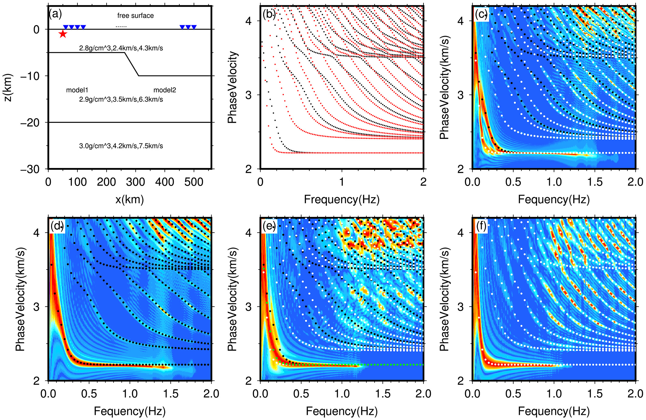
The traditional partitioning method tests various sizes of regular shapes, such as circular or square partitions, to identify suitable configurations and employs moving windows to indiscriminately cover the array. While this approach can be effective in large-scale lithospheric tomography, it presents challenges for imaging complex structures. As noted in previous synthetic work (Li & Chen, 2020) (Figure 1), the dispersion spectrogram obtained using the F-J method bifurcates into different structures’ dispersion patterns when subjected to drastic velocity variations. Therefore, irregular-shaped subarrays are necessary to avoid crossing these areas. Although irregular-shaped partitions can be manually tested and selected, this significantly increases the workload.

Figure 1. A three-dimensional synthetic test for a laterally heterogeneous model. (a) A profile of the test model in the x-z plane. From 0 to 260 km, the thickness of the first layer is 5 km (we call this Model 1); and from 310 to 560 km, the thickness of the first layer is 10 km (we call this Model 2). Between Models 1 and 2, there is a 50-km transition area. We set an earthquake (red star) at a depth of 1 km and 1,000 stations (blue triangles) with an interval of 0.4 km on the free surface. (b) Theoretical dispersion curves of Models 1 and 2. The black points are for Model 1, and the red points are for Model 2. (c) Dispersion spectrum extracted by all records. The black and white points represent the theoretical dispersion curves of Models 1 and 2, respectively (the same in d, e, and f). (d) Dispersion spectrum extracted by the stations from 60 to 250 km along the x axis. (e) Dispersion spectrum extracted by the stations from 200 to 400 km along the x axis. The green points are the fundamental dispersion curves of the average model in the transition area. (f) Dispersion spectrum extracted by the stations from 350 to 500 km

Partition Similarity Test

To address the previously mentioned problem, we aim to develop a quantitative measure for adaptively selecting suitable irregular-shaped partitions. In this study, the proposed measurement is based on the similarity of dispersion curves.

Criteria of similarity between two dispersion curves:

To objectively evaluate dispersion curves’ similarity, a relative error (RE) is defined as follows:

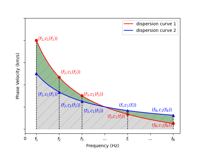
\[e_{12} = \frac{\sum_{i=1}^{N} \left|c_1(f_i)-c_2(f_i)\right|}{\sum_{i=1}^{N}max[c_1(f_i),c_2(f_i)]}\tag{3} \label{eq3})\]

Where \(f_1\) to \(f_N\) represent the N picked frequency points for two dispersion curves, while \(c_1 (f_i)\) and \(c_2 (f_i)\) represent the corresponding phase velocity at \(f_i\). Figure 2 illustrates this design.

Figure 2. An illustration of how relative error is defined for two picked dispersion curves. The red curves and blue curves are two hypothetical dispersion curves. The red dots and blue triangles are hypothetical points from these curves. The green area is absolute error (AE), and the green area divided by the gray area is relative error (RE) between two dispersion curves. The value calculated by \eqref{eq3} approximates RE.

Workflow of the Partition Similarity Test:

The F-J method used a subarray to estimate its centroid one-dimensional velocity structure locally. The idea of the partition similarity test (PST) is to divide the subarray into smaller ones for more local estimation within this subarray and eliminate stations that produce dissimilar dispersion curves to form a new subarray. The workflow consists of four steps:

First, the shape and size of “targets” and “probes” should be established, as shown in Figure 3(a). A “target” refers to a relatively large subarray that is usually directly used for dispersion extraction in the traditional workflow of the F-J method. The shape of targets and probes can be tuned to the array distribution, such as a circle or square. Appropriate sizes of targets need to be tested to produce a better dispersion spectrogram, the same as previous applications usually do. A helpful starting point is applying the F-J method to the entire array, with the first bifurcation revealed by the dispersion spectrogram indicating the lower limit of the resolvable frequency range. Targets are fixed-shape arrays with sufficient aperture to capture this minimum frequency band \((f_{min})\). The dispersion at f_min can be accurately estimated by the F-J method ddependingon the aperture \((r_{max})\) of the array, which is considered at least half of the wavelength (\(\lambda_{max}\)) at the \(f_{min}\) in this study:

\[r_{max} \geq \frac{\lambda_{max}}{2} = \frac{c(f_{min})}{2\cdot f_{min}} \tag{4} \label{eq4}\]

“Probes” are smaller subarrays with centroids located within a target. These provide more localized dispersion estimations around the target. The probe size is determined by the bifurcation frequency range (i.e., \(f_{1}\) to \(f_{N}\)) of the target’s dispersion spectrogram (Figure 3(b)), ensuring accurate dispersion extraction using the same criteria as above.
Second, the relative error (RE) of each probe is calculated within the target by comparing its dispersion curve against that of the reference probe, the one nearest to the target’s centroid. As shown in Figures 3(a) and 3(b), probes with similar velocity models will produce comparable dispersion curves (e.g., Probe B in Figure 3(a)), while dissimilar ones (e.g., Probes C and D in Figure 3(b)) will exhibit larger RE values.
Third, an error threshold is established, and probes with small RE values are combined into a new, larger subarray. For this study, probes in cyan in Figure 3(c) represent those with RE values below the empirically set threshold of 0.05, forming the refined subarray. The robustness of this threshold is discussed in a subsequent section.
Finally, quality control is applied to remove or adjust unsatisfactory subarrays. In transition zones, some probes may still show bifurcation in their dispersion spectrograms (e.g., when Probe C in Figure 3(a) is servered as the reference probe as Probe A), resulting in the acceptance of only a few or disconnected probes. Therefore, only subarrays formed by more than four adjacent probes are retained for analysis. Additionally, the F-J spectrograms of these new subarrays are examined to confirm that bifurcation is mitigated. For subarrays that remain unsatisfactory, error thresholds between 0.02 and 0.1 will be applied and tested again to address specific cases.

Figure 3. Illustration of the Partition Similarity Test (PST) concept. (a) Target and Probe Definition: In the F-J method, the cross-correlation functions (CCFs) of a seismic station array are used to estimate the velocity structure at its centroid. The "target" refers to a relatively large seismic station array (black hollow circles) spanning multiple one-dimensional velocity structures (orange and green background regions). The target can be divided into smaller subarrays, called "probes" (e.g., three-station groups in this case), which enable localized dispersion curve extraction around the target centroid. Among these, the probe closest to the target centroid is designated as the reference probe (Probe A). The relative error (RE) of all other probes is calculated with respect to Probe A. Probes with the same velocity structure as Probe A are marked in cyan, those spanning two structures are marked in yellow, and those covering a different structure are marked in red. (b) Relative Error (RE) Calculation: This panel illustrates the RE calculation and a hypothetical fundamental mode dispersion curve distributions of the probes in (a). Red dots and blue triangles represent dispersion points from an outlier and the reference probe, respectively. The gray "slashed" area denotes the absolute error (AE) between the curves. Dividing the AE by the gray area is defined as the RE, as approximated by equation (3). (c) New Subarray Formation: Probes with similar dispersion curves (cyan centroids in (a) and corresponding cyan curves in (b)) are combined to form a new subarray. Note that this process excludes certain stations from the target, causing a centroid shift in the new subarray.

Comparison to F-J

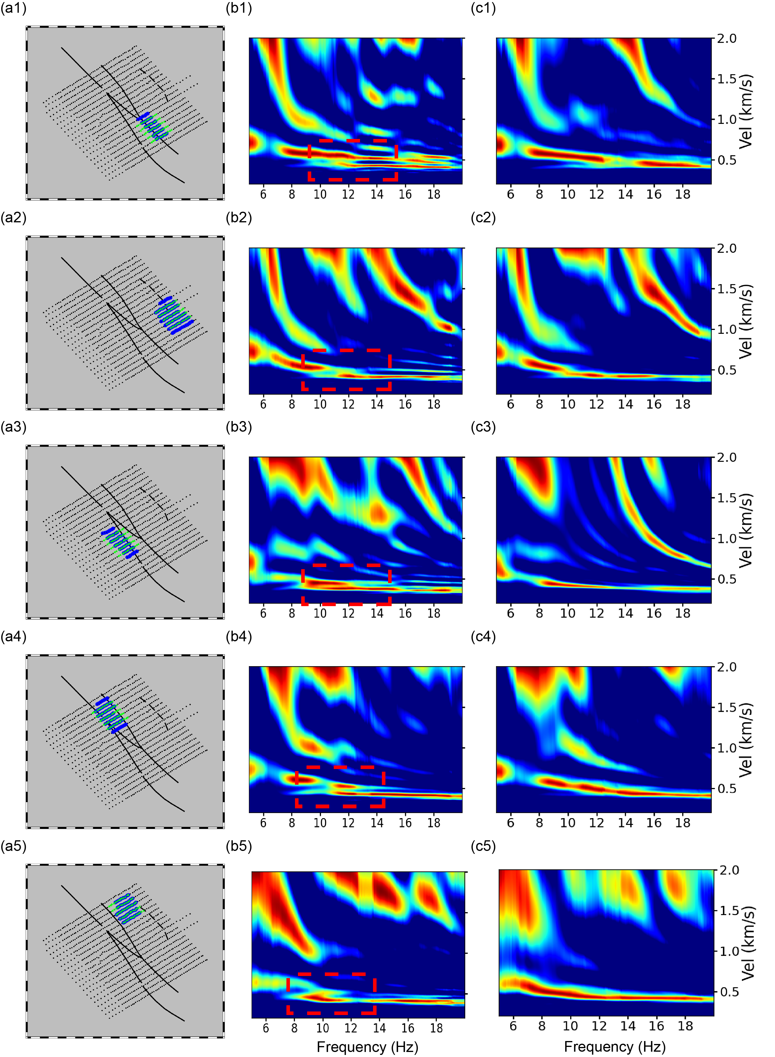
Here, we demonstrate the effectiveness of the FJ-PST by comparing it to the dispersion spectrogram calculated by the traditional F-J method in a dense nodal array deplyed at San Jacinto Fault Zone (Ben-Zion et al., 2015). As indicated in Figure 4, the entire array suffered from extensive and severe fundamental mode bifurcation on the dispersion spectrogram calculated by the traditional F-J method, while the FJ-PST successfully detected the boundaries and adaptively adjusted the subarrays to mitigate this issue.

Figure 4. The comparison between FJ-PST and the traditional F-J for 5 different subarrays. (a) The subarrays of FJ-PST (blue) and the nearest subarrays of traditional F-J (green). (b) The dispersion spectrogram calculated by the F-J for the green subarrays in (a). The red dashed squares indicate the fundamental mode bifurcation. (c) The dispersion spectrogram calculated by the F-J for the blue subarrays in (a).

Applications

High-resolution Fault-Zone Tomography

Related Project: Complex Fault Tomography Using FJ-PST (San Jacinto Fault Zone)